Getting Started with PrestoDB and Aria Scan Optimizations

PrestoDB recently released a set of experimental features under their Aria project in order to increase table scan performance of data stored in ORC files via the Hive Connector. In this post, we’ll check out these new features at a very basic level using a test environment of PrestoDB on Docker. To find out more about the Aria features, you can check out the Facebook Engineering blog post which was published June 2019.

Presto is a massively parallel processing (MPP) SQL execution engine. The execution engine is decoupled from data storage, and the project contains numerous plugins, called Connectors, that provide the Presto engine with data for query execution. Data is read from the data store, then handed to Presto where it takes over to perform the operations of the query, such as joining data and performing aggregations. This decoupling of data storage and execution allows for a single Presto instance to query various data sources, providing a very powerful federated query layer. There are many connectors available for Presto, and the community regularly provides additional connectors for data stores.

The Hive Connector is often considered the standard connector for Presto. This connector is configured to connect to a Hive Metastore, which exposes metadata about the tables defined in the Metastore. Data is typically stored in HDFS or S3, and the Metastore provides information about where the files are stored and in what format; typically ORC but other supported formats like Avro and Parquet are supported. The Hive connector allows the Presto engine to scan data from HDFS/S3 in parallel into the engine to execute your query. ORC (Optimized Row Columnar) format is a very standard and common format for storing data, as it provides good compression and performance.

Presto has two core services for executing queries. A Coordinator, which is responsible for query parsing and scheduling (among other things), and many Workers which execute the queries in parallel. The Coordinator can also act as a Worker, though it is not used for production environments. Since we’re playing with Presto here, we’ll just use one node to act as both a Coordinator and Worker. More detailed documentation, including installation details, can be found here .

Let’s take a look at getting a Docker image together for Presto (though they already exist on Dockerhub, e.g. ahanaio/prestodb-sandbox ). We can see below how relatively easy it is to get Presto up and running. We download Presto, copy some configuration files in a local etc directory into the image, and specify an entry point to run the server.

FROM openjdk:8-jre

# Pick our Presto Version and the URL to download
ARG PRESTO_VERSION=0.235.1
ARG PRESTO_BIN=https://repo1.maven.org/maven2/com/facebook/presto/presto-server/${PRESTO_VERSION}/presto-server-${PRESTO_VERSION}.tar.gz

# Update the base image OS and install wget and python
RUN apt-get update
RUN apt-get install -y wget python

# Download Presto and unpack it to /opt/presto
RUN wget --quiet ${PRESTO_BIN}
RUN mkdir -p /opt
RUN tar -xf presto-server-${PRESTO_VERSION}.tar.gz -C /opt
RUN rm presto-server-${PRESTO_VERSION}.tar.gz
RUN ln -s /opt/presto-server-${PRESTO_VERSION} /opt/presto

# Copy configuration files on the host into the image
COPY etc /opt/presto/etc

# Download the Presto CLI and put it in the image
RUN wget --quiet https://repo1.maven.org/maven2/com/facebook/presto/presto-cli/${PRESTO_VERSION}/presto-cli-${PRESTO_VERSION}-executable.jar
RUN mv presto-cli-${PRESTO_VERSION}-executable.jar /usr/local/bin/presto
RUN chmod +x /usr/local/bin/presto

# Specify the entrypoint to start
ENTRYPOINT /opt/presto/bin/launcher run

There are four files in the etc folder to configure Presto, along with two catalogs. Details of them can be found here . They are:

etc/
├── catalog
│   ├── hive.properties  # Defines configuration properties for our Hive Metastore
│   └── tpch.properties  # Enables the TPCH connector to generate data
├── config.properties 	 # Presto instance configuration properties
├── jvm.config           # JVM configuration for the process
├── log.properties       # Logging configuration
└── node.properties      # Node-specific configuration properties

The four files directly under etc are documented in the above link. Let’s look at the details of the two catalogs: hive and tpch. The former will be used to read data, and the latter will be used to generate data into our Hive warehouse to run queries. Setting up Hive is outside the scope of this document, but will be covered in a future post. In short, you need a catalog service in order to use the Hive connector, such as a Hive Metastore or AWS Glue. The catalog service contains all of the table definitions used by Presto, and data is typically stored in HDFS or S3. We’ve set up a Dockerized Hive Metastore and single-node HDFS instance.

etc/catalog/hive.properties

connector.name=hive-hadoop2
hive.metastore.uri=thrift://localhost:9083/hivemetastore
hive.metastore.username=hive
hive.allow-drop-table=true

etc/catalog/tpch.properties

connector.name=tpch

We’re now ready to build our Docker container and start Presto using host networking so it can talk to the Metastore and HDFS which is running on the host (also in Docker).

docker build . -t prestodb:latest
docker run --name presto --network host prestodb:latest

We’ll use the Presto CLI to connect to Presto that we put inside the image.

docker exec -it presto presto

Next, we will create our schema to hold the TPC-H data set and then create the tables. By default, Presto will create ORC files, which is convenient for us since that is what we’re looking at testing. We are using the sf100 TPC-H schema to create a data set of about 23 GB total. This should give us enough data to show off the Aria enhancements. (The sf stands for scale factor and is about 100 times larger than the sf1 schema.)

CREATE SCHEMA hive.tpch;

CREATE TABLE hive.tpch.customer AS SELECT * FROM tpch.sf100.customer;
CREATE TABLE hive.tpch.lineitem AS SELECT * FROM tpch.sf100.lineitem;
CREATE TABLE hive.tpch.nation AS SELECT * FROM tpch.sf100.nation;
CREATE TABLE hive.tpch.orders AS SELECT * FROM tpch.sf100.orders;
CREATE TABLE hive.tpch.part AS SELECT * FROM tpch.sf100.part;
CREATE TABLE hive.tpch.partsupp AS SELECT * FROM tpch.sf100.partsupp;
CREATE TABLE hive.tpch.region AS SELECT * FROM tpch.sf100.region;
CREATE TABLE hive.tpch.supplier AS SELECT * FROM tpch.sf100.supplier;

USE tpch;

Let’s talk a bit about how Presto executes a query. The Presto Coordinator parses the query to build a plan (which we will see examples of below). Once the plan is made, it is broken into several stages (or fragments) which execute a series of operators. Operators are a particular function that the engine performs to execute your query. This typically begins with scanning data via a Connector, then performing operations such as filtering data, partial aggregations, and commonly exchanging data between Presto workers to perform joins and final aggregations. All of these stages are broken into splits, which is a unit of parallelism in Presto. Workers execute a configurable number of splits in parallel to get your desired results. All data in the engine is kept in-memory (as long as you don’t go past the thresholds of the cluster; another topic for another time).

The Hive connector (and all connectors for that matter) are responsible for breaking the input data set into splits for Presto to read in parallel. As an optimization, the Presto engine will tell connectors the predicates used in a query and what columns are being selected, called predicate pushdown, which enables connectors to drop data before even handing it to the engine (what this blog post is all about!).

To demonstrate the predicate pushdown, let’s take a look at a basic query – counting rows of a table within a range. The TPC-H lineitem table has about 600 million rows with a shipdate between 1992 and 1998. Let’s start without enabling the session properties to enable the Aria enhancements, running an EXPLAIN command to take a look at the query plan.

presto:tpch> EXPLAIN (TYPE DISTRIBUTED) SELECT COUNT(shipdate) FROM lineitem WHERE shipdate BETWEEN DATE '1992-01-01' AND DATE '1992-12-31';

Fragment 0 [SINGLE]
    Output layout: [count]
    Output partitioning: SINGLE []
    Stage Execution Strategy: UNGROUPED_EXECUTION
    - Output[_col0] => [count:bigint]
            _col0 := count
        - Aggregate(FINAL) => [count:bigint]
                count := ""presto.default.count""((count_4))
            - LocalExchange[SINGLE] () => [count_4:bigint]
                - RemoteSource[1] => [count_4:bigint]

Fragment 1 [SOURCE]
    Output layout: [count_4]
    Output partitioning: SINGLE []
    Stage Execution Strategy: UNGROUPED_EXECUTION
    - Aggregate(PARTIAL) => [count_4:bigint]
            count_4 := ""presto.default.count""((shipdate))
        - ScanFilter[table = TableHandle {connectorId='hive', connectorHandle='HiveTableHandle{schemaName=tpch, tableName=lineitem, analyzePartitionValues=Optional.empty}', layout='Optional[tpch.lineitem{domains={shipdate=[ [[1992-01-01, 1992-12-31]] ]}}]'}, grouped = false, filterPredicate = shipdate BETWEEN (DATE 1992-01-01) AND (DATE 1992-12-31)] => [shipdate:date]
                Estimates: {rows: 600037902 (2.79GB), cpu: 3000189510.00, memory: 0.00, network: 0.00}/{rows: ? (?), cpu: 6000379020.00, memory: 0.00, network: 0.00}
                LAYOUT: tpch.lineitem{domains={shipdate=[ [[1992-01-01, 1992-12-31]] ]}}
                shipdate := shipdate:date:10:REGULAR

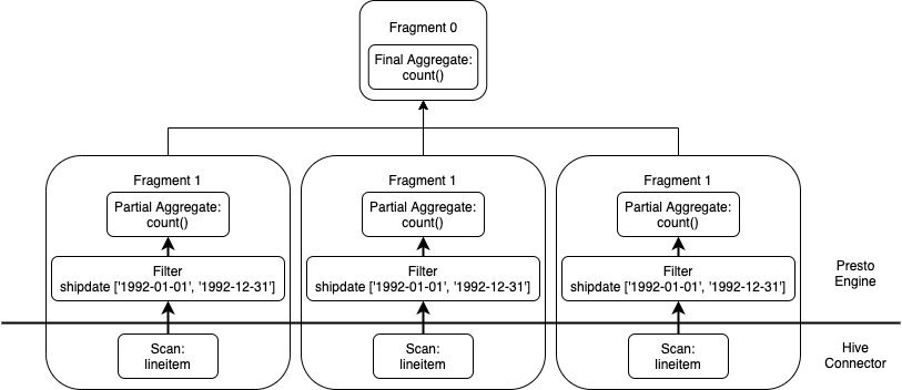
Query plans are read bottom-up, starting with Fragment 1 that will scan the lineitem table in parallel, performing the filter on the shipdate column to apply the predicate. It will then perform a partial aggregation for each split, and exchange that partial result to the next stage Fragment 0 to perform the final aggregation before delivering the results to the client. In an effort to visualize the plan, see below. Note the horizontal line towards the bottom of the diagram, indicating which code executes in the Hive Connector and which code executes in the Presto engine.

We’ll now execute this query!

presto:tpch> SELECT COUNT(shipdate) FROM lineitem WHERE shipdate BETWEEN DATE '1992-01-01' AND DATE '1992-12-31';
  _col0   
----------
 76036301
(1 row)

Query 20200609_154258_00019_ug2v4, FINISHED, 1 node
Splits: 367 total, 367 done (100.00%)
0:09 [600M rows, 928MB] [63.2M rows/s, 97.7MB/s]

We see there are a little over 76 million rows lineitem table in the year 1992. It took about 9 seconds to execute this query, processing 600 million rows.

Now let’s set the session properties pushdown_subfields_enabled and hive.pushdown_filter_enabled to enable the Aria features and take a look at the same explain plan.

presto:tpch> SET SESSION pushdown_subfields_enabled=true;
SET SESSION
presto:tpch> SET SESSION hive.pushdown_filter_enabled=true;
SET SESSION
presto:tpch> EXPLAIN (TYPE DISTRIBUTED) SELECT COUNT(shipdate) FROM lineitem WHERE shipdate BETWEEN DATE '1992-01-01' AND DATE '1992-12-31';
Fragment 0 [SINGLE]
    Output layout: [count]
    Output partitioning: SINGLE []
    Stage Execution Strategy: UNGROUPED_EXECUTION
    - Output[_col0] => [count:bigint]
            _col0 := count
        - Aggregate(FINAL) => [count:bigint]
                count := ""presto.default.count""((count_4))
            - LocalExchange[SINGLE] () => [count_4:bigint]
                - RemoteSource[1] => [count_4:bigint]

Fragment 1 [SOURCE]
    Output layout: [count_4]
    Output partitioning: SINGLE []
    Stage Execution Strategy: UNGROUPED_EXECUTION
    - Aggregate(PARTIAL) => [count_4:bigint]
            count_4 := ""presto.default.count""((shipdate))
        - TableScan[TableHandle {connectorId='hive', connectorHandle='HiveTableHandle{schemaName=tpch, tableName=lineitem, analyzePartitionValues=Optional.empty}', layout='Optional[tpch.lineitem{domains={shipdate=[ [[1992-01-01, 1992-12-31]] ]}}]'}, grouped = false] => [shipdate:date]
                Estimates: {rows: 540034112 (2.51GB), cpu: 2700170559.00, memory: 0.00, network: 0.00}
                LAYOUT: tpch.lineitem{domains={shipdate=[ [[1992-01-01, 1992-12-31]] ]}}
                shipdate := shipdate:date:10:REGULAR
                    :: [[1992-01-01, 1992-12-31]]

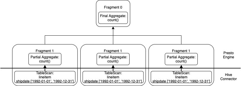
Note the major difference in the query plan at the very bottom, the inclusion of shipdate column in the TableScan operation. We see here that the connector now notices the predicate on the shipdate column of 1992-01-01 to 1992-12-31. To visualize, we see this predicate is pushed down to the connector, removing the necessity of the engine to filter this data.

We’ll run this query again!

presto:tpch> SELECT COUNT(shipdate) FROM lineitem WHERE shipdate BETWEEN DATE '1992-01-01' AND DATE '1992-12-31';
  _col0   
----------
 76036301
(1 row)

Query 20200609_154413_00023_ug2v4, FINISHED, 1 node
Splits: 367 total, 367 done (100.00%)
0:05 [76M rows, 928MB] [15.5M rows/s, 189MB/s]

We get the same result running the query, but the query time took almost half as long and, more importantly, we see only 76 million rows were scanned! The connector has applied the predicate on the shipdate column, rather than having the engine process the predicate. This saves some CPU cycles, resulting in faster query results. YMMV for your own queries and data sets, but if you’re using the Hive connector with ORC files, it is definitely worth a look.